Chapter 2. Pulsar Observing Techniques

Pulsar discovery immediately triggered a wave of theoretical and observational work. One of the key lessons from the Cambridge discovery was that pulsar observations require radio telescopes with both high sensitivity and high time resolution. Once that became clear, large instruments such as the 305-m Arecibo telescope, the 76-m Jodrell Bank telescope, and the 64-m Parkes telescope became much more effective than the original Cambridge array for pulsar work.

1. The sensitivity problem

The progress achieved in pulsar observing has been extraordinary. More than one thousand pulsars had already been discovered by the time of the source text, including more than fifty millisecond pulsars, many radio pulsar binaries, systems with planetary companions, pulsars visible in X-rays and $\gamma$ rays, and many pulsars associated with supernova remnants.

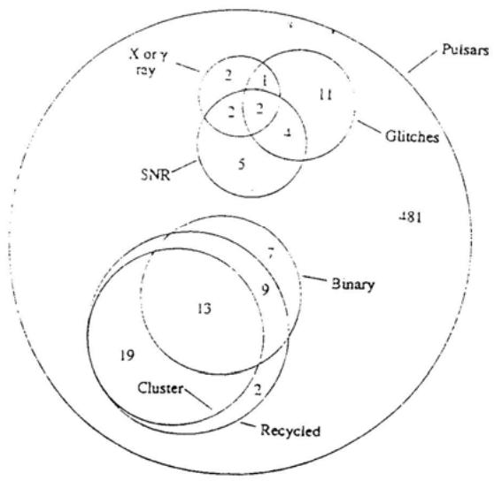Figure 2.1. Classification of 558 pulsars. The horizontal direction roughly tracks increasing period, while the vertical direction tracks increasing period derivative.

For radio pulsar observations, the minimum detectable flux density can be written as

$$S _ {\min } = \frac {C \left(T _ {\text {sys}} + T _ {\text {sky}}\right)}{G \sqrt {N _ {p} t _ {\text {int}} \Delta \nu}} \sqrt {\frac {W}{P - W}}.$$

Here:

• $S_{\min}$ is the observing sensitivity
• $C$ is the required signal-to-noise threshold
• $T_{\text{sys}}$ is the system noise temperature
• $T_{\text{sky}}$ is the sky background temperature
• $G$ is the antenna gain
• $N_p$ is the number of polarizations used
• $\Delta \nu$ is the total bandwidth
• $t_{\text{int}}$ is the observing time
• $P$ is the pulsar period
• $W$ is the effective pulse width

The pulse width itself is broadened by several effects:

$$W^2 = W_0^2 + t_{\text{samp}}^2 + t_{DM}^2 + t_{\text{scatt}}^2,$$

where $W_0$ is the intrinsic pulse width, $t_{\text{samp}}$ is the sampling interval, $t_{DM}$ is dispersion broadening across the channel bandwidth, and $t_{\text{scatt}}$ is broadening caused by interstellar scattering.

The text gives the approximate relations

$$t_{\text{scatt}} = \left(\frac{DM}{1000}\right)^{3.5}\left(\frac{400}{\nu_{\text{MHz}}}\right)^4,$$ $$t_{DM} = 4.15 \times 10^3 \frac{DM}{\nu_{\text{MHz}}^2},$$ $$DM = \int_0^d n_e\,dl \approx \bar n_e d.$$

These relations show immediately why distant, high-DM pulsars are difficult to detect, especially at low frequency. Broadening grows rapidly with dispersion measure and falls with observing frequency, so high-frequency observations can compensate for some of the propagation smearing.

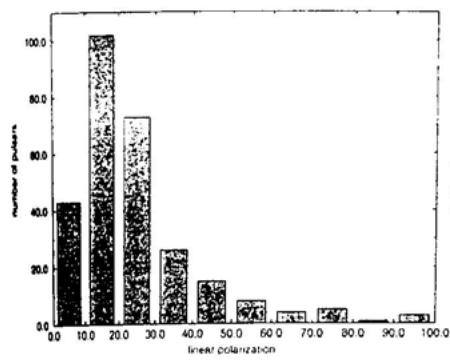
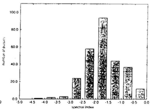
Most pulsars are faint. In the 556-source 400-MHz sample discussed in the text, nearly half had flux densities below 5 mJy, while only a tiny fraction exceeded 50 mJy. Since pulsars also have steep radio spectra, they are often even fainter at higher frequencies.

The original chapter groups pulsar observing into three broad goals:

• surveys to discover more pulsars
• timing observations to measure periods, derivatives, glitches, orbital parameters, ages, magnetic fields, and related quantities
• intensity and polarization observations of mean profiles, subpulses, micropulses, and single pulses

The last of these places the highest demand on sensitivity. Some polarization work requires signal-to-noise ratios near 100, far above what is needed for ordinary timing.

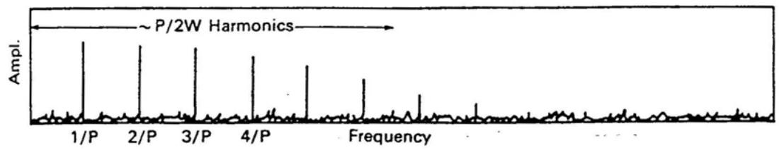
2. Building large radio telescopes to improve sensitivity

Astronomical observations need not only sensitivity but also angular resolution. In general, the angular resolution of a telescope scales like

$$\theta \sim 1.22 \frac{\lambda}{D},$$

where $D$ is the effective aperture size. Pulsar work, however, usually values sensitivity more than fine imaging resolution. Except for special studies of very bright pulsars, it does not matter too much if several pulsars fall inside one beam. What matters most is collecting enough signal.

That is why large single-dish radio telescopes became the main instruments of pulsar astronomy. The text discusses major instruments such as Effelsberg, Green Bank, Arecibo, Jodrell Bank, and Parkes, as well as phased arrays and synthesis instruments used in coherent-sum mode.

The original discussion also highlights larger strategic plans:

• medium-scale national telescopes that would close sensitivity gaps
• the proposed 500-m FAST telescope in Guizhou
• the international idea of an even larger square-kilometre-scale radio array

From a pulsar point of view, the scientific payoff of such telescopes is not only the discovery of more pulsars, but the discovery of new classes of pulsars. As the known sample grew from a few hundred to many hundreds, the population diversified into millisecond pulsars, double-neutron-star systems, neutron-star/white-dwarf systems, high-mass companions, pulsars with planets, and high-energy pulsars.

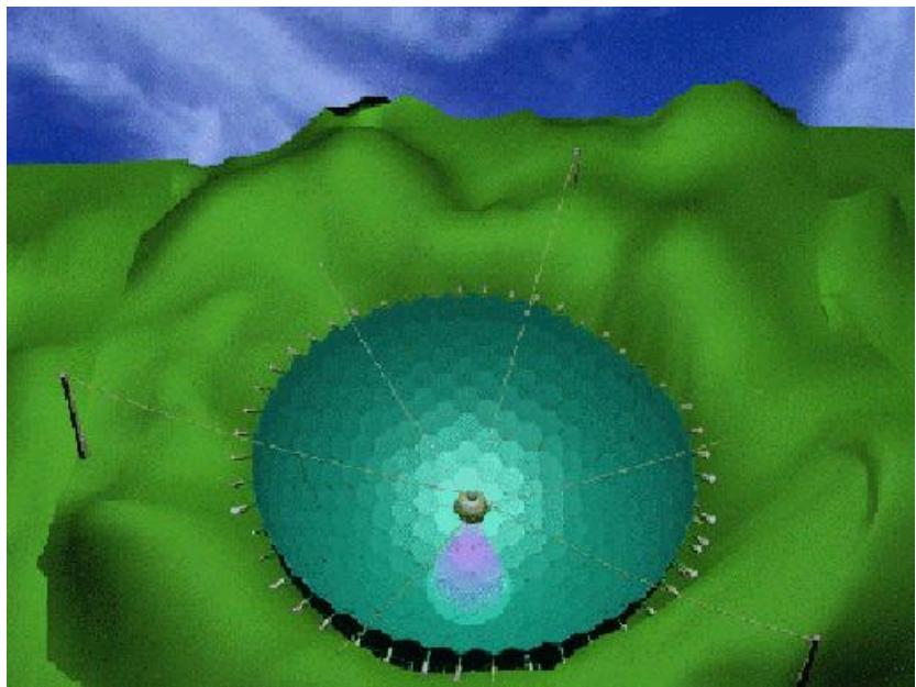Figure 2.2. Concept drawing for the planned 500-m telescope in Guizhou.

The chapter also includes a historical table of major pulsar surveys, showing how different telescopes, frequencies, and observing strategies led to successive jumps in the number of discoveries.

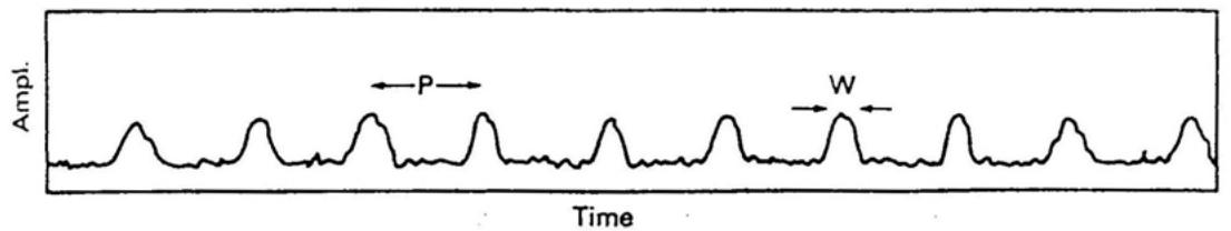
3. Improving sensitivity by folding at the pulse period

To record pulse structure directly, the receiver time constant must be shorter than the pulsar period, often only a tenth of the period or less. For millisecond pulsars, survey sampling times may need to be as short as 0.1 ms or even less. That requirement sharply reduces raw sensitivity, because sensitivity scales only as the square root of integration time.

The key way around this is folding. Signal and noise add differently:

• coherent signal aligned at the correct phase adds linearly
• random noise grows only as the square root of the number of samples

If data are folded at the pulsar period and summed, the signal-to-noise ratio increases substantially. The profile produced by this process is the mean pulse profile. It represents the long-term stable emission geometry and is essential for pulsar analysis.

This is not only a sensitivity trick. Folding is the fundamental step that produces the mean pulse profile itself. Even for strong pulsars, many pulses must be combined to obtain the stable average shape used in scientific interpretation.

The chapter also notes an important limitation: this technique cannot be used for studies that depend on genuine pulse-to-pulse variability, such as drifting subpulses or micropulses. Those observations can only be carried out for relatively strong pulsars.

4. Dedispersion receiver technology

Sensitivity can also be improved by increasing bandwidth. Since sensitivity scales with the square root of bandwidth, a hundredfold increase in bandwidth yields a tenfold increase in sensitivity. But interstellar dispersion prevents us from simply making the receiver arbitrarily wideband.

Different radio frequencies propagate at different group velocities in the ionized interstellar medium, so low-frequency radiation arrives later than high-frequency radiation. If the bandwidth is too wide, the pulse is smeared so strongly that its structure is washed out or even erased.

The upper limit on the channel bandwidth can be written as

$$B_i = \frac{\nu_{\text{MHz}}^3}{8.3 \times 10^3 DM}\tau,$$

where $\tau$ is the pulse width. The physical meaning is that the dispersion smearing across one channel must not exceed the pulse width itself.

For some pulsars, even a 1-MHz channel is too wide. The Crab pulsar, observed at 232 MHz, would show a delay across a 1-MHz band of about 39.4 ms, already longer than its 33-ms period. In that case the allowed channel width is only about 33 kHz.

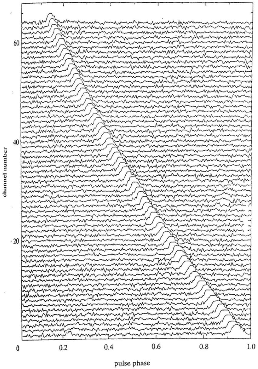Figure 2.3a. Example of a dispersed pulsar signal, with the high-frequency pulse arriving earlier than the low-frequency pulse.

The dedispersion receiver solves this by splitting the full band into many narrow channels. Each channel is narrow enough to keep intra-channel smearing tolerable, and then the output channels are delayed by the proper amounts and summed to reconstruct a much cleaner pulse.

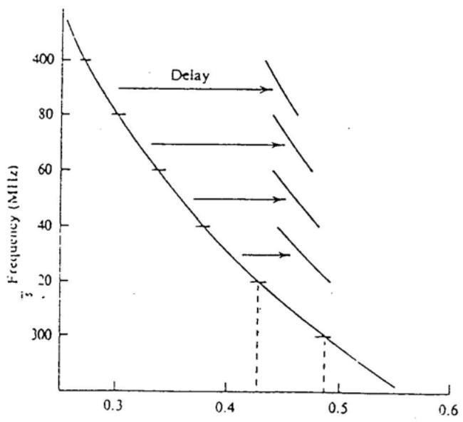Figure 2.3b. Basic principle of dedispersion.

The text gives several examples from Parkes and Urumqi showing how powerful multichannel dedispersion systems dramatically increased effective sensitivity. A large gain in bandwidth can be as valuable as building a much larger telescope.

5. Pulsar search strategy

The final part of the chapter turns from hardware to search design. Pulsar searching is not just "point and observe." A survey has to make explicit choices about target region, frequency, beam pattern, sky coverage, and processing pipeline.

5.1 Defining a survey

The first step is deciding what region of the sky to search and which kind of pulsars to prioritise. This depends on:

• observing frequency
• telescope beam size
• total sky coverage
• sensitivity to short periods
• expected dispersion and scattering in the survey region

Surveys near the Galactic plane, for example, contain rich pulsar populations but also high dispersion and scattering.

5.2 Single-beam and multibeam surveys

The text compares traditional single-beam surveys with multibeam systems. Multibeam receivers greatly improve survey speed because many adjacent sky positions can be observed simultaneously. This is one reason the Parkes multibeam survey was so successful.

5.3 High-frequency surveys

High-frequency surveys can outperform low-frequency ones in strongly scattered regions because propagation broadening drops steeply with frequency. Although pulsars are fainter at high frequency, the reduced smearing can more than compensate for that in some parts of the sky.

5.4 Survey technology

The source text ends with a survey-technology discussion that includes filterbanks, multichannel dedispersion, short integration pipelines, candidate selection, and the continual drive toward lower detectable flux densities.

The central message of the chapter is clear: pulsar observing is an optimisation problem in which telescope aperture, receiver noise, bandwidth, dedispersion capability, sampling time, and survey design must all be balanced together. Pulsars are not merely faint radio sources. They are faint, rapidly varying, propagation-distorted radio sources, and every major advance in pulsar astronomy has come from improving our ability to handle that full combination.